How To Create A Filter In Excel

Lesson 19: Filtering Data

/en/excel2013/sorting-data/content/

Introduction

If your worksheet contains a lot of content, it can be difficult to observe information quickly. Filters can exist used to narrow downwards the data in your worksheet, assuasive you to view only the data you demand.

Optional: Download our practice workbook.

To filter data:

In our example, we'll utilize a filter to an equipment log worksheet to display only the laptops and projectors that are available for checkout.

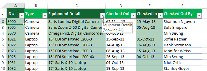
In order for filtering to piece of work correctly, your worksheet should include a header row, which is used to identify the proper noun of each column. In our instance, our worksheet is organized into unlike columns identified by the header cells in row 1: ID#, Type, Equipment Particular, and and so on.
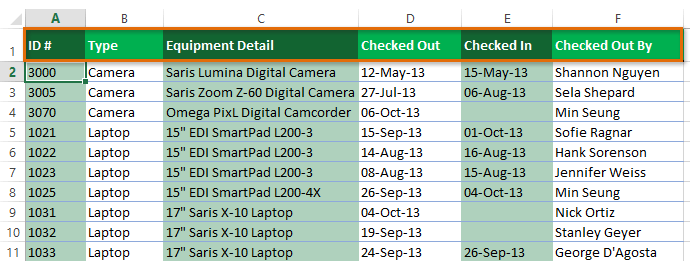A worksheet with a header row
Select the Information tab, so click the Filter command.
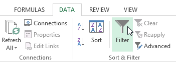Clicking the Filter control
A drop-downwardly arrow will appear in the header cell for each column.
Click the drop-downwardly arrow for the cavalcade y'all desire to filter. In our example, we will filter cavalcade B to view just sure types of equipment.
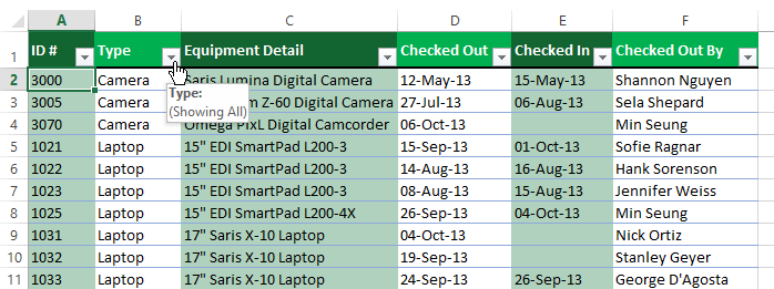Clicking the driblet-down arrow for column B
The Filter menu will appear.
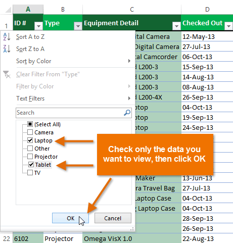
Uncheck the box next to Select All to apace deselect all data.
Unchecking Select All
Check the boxes next to the data you want to filter, then click OK. In this example, we will cheque Laptop and Tablet to view just those types of equipment.
Choosing data to filter and clicking OK
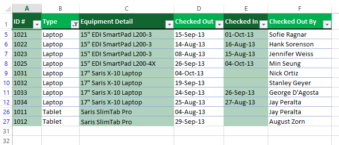
The data will exist filtered, temporarily hiding any content that doesn't match the criteria. In our example, only laptops and tablets are visible.
The filtered information

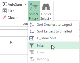
Filtering options can likewise be accessed from the Sort & Filter control on the Home tab.

Screenshot of Excel 2013 Accessing Filter options from the Domicile tab

To employ multiple filters:

Filters are cumulative, which means you can apply multiple filters to assistance narrow down your results. In this case, we've already filtered our worksheet to show laptops and projectors, and we'd similar to narrow information technology downward further to simply evidence laptops and projectors that were checked out in Baronial.

Click the drop-down arrow for the column you desire to filter. In this case, we will add a filter to column D to view information by date.
Clicking the drib-downwards arrow for column D
The Filter menu will announced.
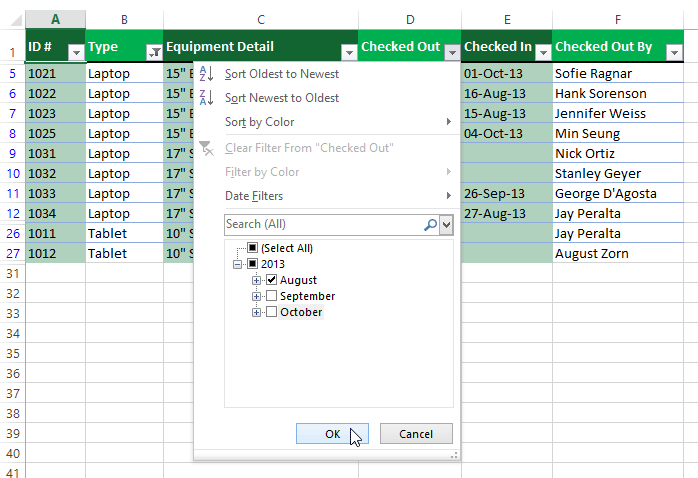
Bank check or uncheck the boxes depending on the data you want to filter, and so click OK. In our example, we'll uncheck everything except for August.
Choosing data to filter and clicking OK
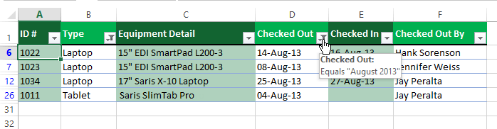
The new filter will be applied. In our instance, the worksheet is now filtered to testify simply laptops and tablets that were checked out in August.
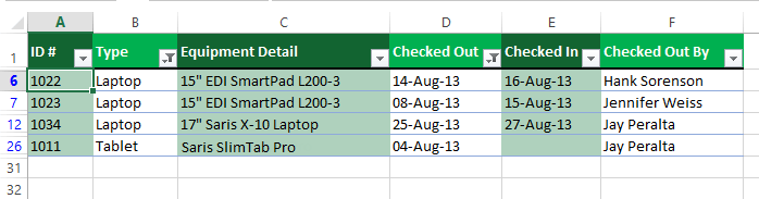The filtered data

To clear a filter:

Afterward applying a filter, you may want to remove—or clear—it from your worksheet so you'll be able to filter content in different ways.

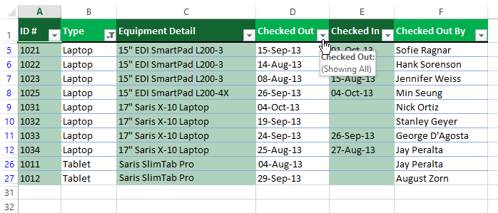
Click the drop-down pointer for the filter you lot desire to clear. In our instance, nosotros'll clear the filter in cavalcade D.
Clicking the drop-downwardly arrow for column D
The Filter menu will appear.
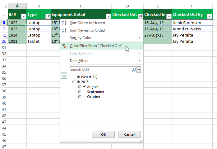
Cull Clear Filter From [Cavalcade NAME] from the Filter menu. In our case, nosotros'll select Clear Filter From "Checked Out".
Clearing a filter
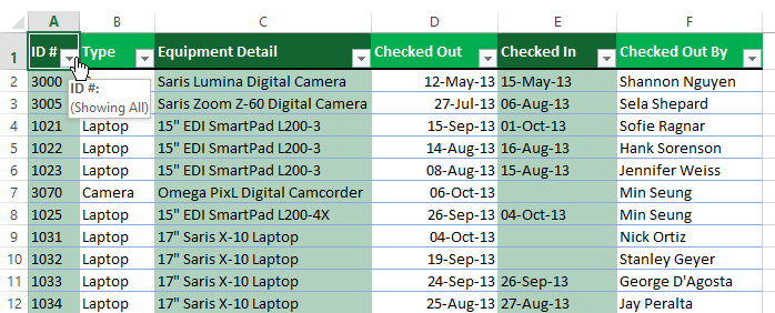
The filter will be cleared from the column. The previously hidden data volition be displayed.
The cleared filter

To remove all filters from your worksheet, click the Filter control on the Data tab.

Screenshot of Excel 2013 Clicking the Filter command to remove filters

Advanced filtering

If you need to filter for something specific, basic filtering may not requite you enough options. Fortunately, Excel includes many advanced filtering tools, including search, text, date, and number filtering, which tin can narrow your results to help find exactly what yous need.

To filter with search:

Excel allows yous to search for data that contains an exact phrase, number, engagement, and more than. In our case, we'll use this feature to prove only Saris brand products in our equipment log.

Select the Information tab, then click the Filter control. A driblet-downwardly arrow will announced in the header cell for each column. Note: If y'all've already added filters to your worksheet, you tin skip this footstep.
Click the driblet-down arrow for the column you want to filter. In our case, we'll filter column C.
Clicking the driblet-down arrow for column C
The Filter carte will appear. Enter a search term into the search box. Search results will appear automatically beneath the Text Filters field as you type. In our example, we'll type saris to find all Saris brand equipment.
When you're done, click OK.
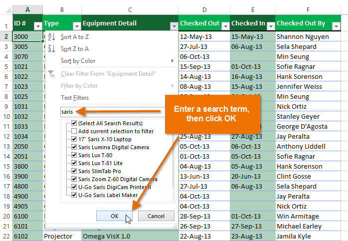Entering a search term and clicking OK
The worksheet volition be filtered according to your search term. In our case, the worksheet is now filtered to show only Saris make equipment.
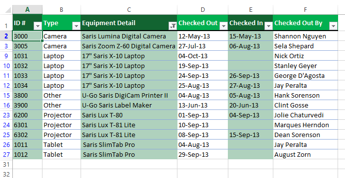The worksheet filtered by the search term

To utilize avant-garde text filters:

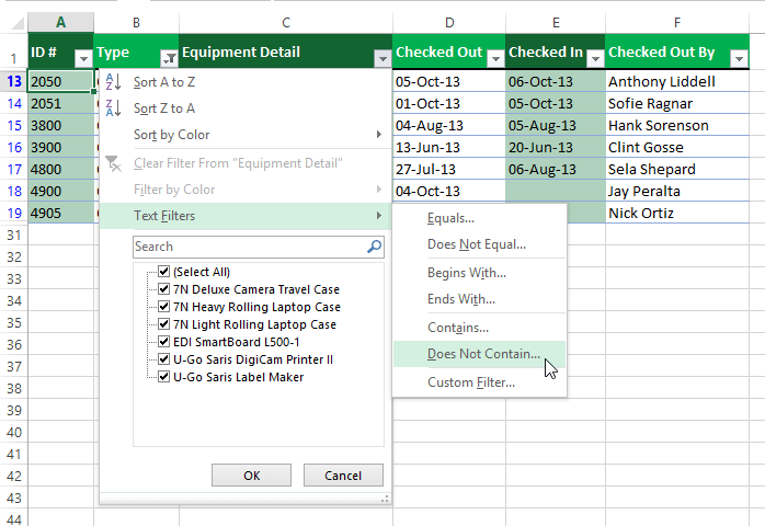
Avant-garde text filters can exist used to display more specific information, such every bit cells that contain a certain number of characters, or information that excludes a specific word or number. In our instance, we've already filtered our worksheet to simply show items with O ther in the Blazon column, only we'd like to exclude any item containing the discussion example.

Select the Information tab, and then click the Filter command. A drop-downwardly arrow volition announced in the header cell for each column. Note: If you lot've already added filters to your worksheet, yous can skip this footstep.
Click the driblet-down arrow for the cavalcade yous want to filter. In our example, we'll filter column C.
Clicking the drop-downward pointer for column C
The Filter carte du jour volition appear. Hover the mouse over Text Filters, then select the desired text filter from the driblet-downward carte du jour. In our case, we'll choose Does Not Comprise... to view data that does not contain specific text.
Selecting a text filter
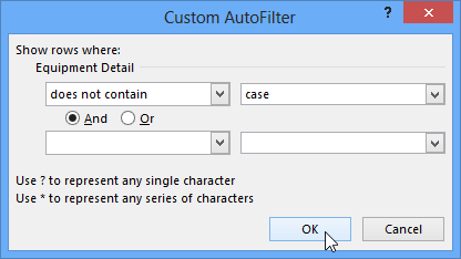
The Custom AutoFilter dialog box will appear. Enter the desired text to the correct of the filter, then click OK. In our example, we'll type instance to exclude any items containing this give-and-take.
Applying a text filter
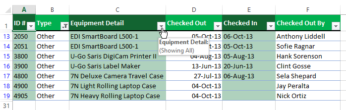
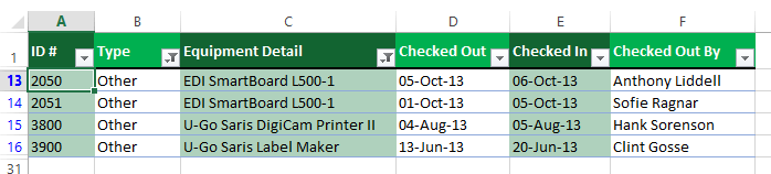
The data will be filtered by the selected text filter. In our example, our worksheet now displays items in the Other category that practice not contain the give-and-take case.
The applied text filter

To utilize avant-garde date filters:

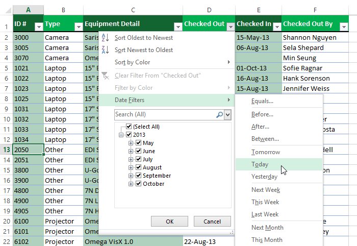
Advanced engagement filters tin can be used to view data from a sure fourth dimension menstruation, such as last twelvemonth, side by side quarter, or betwixt two dates. In this example, we will use advanced engagement filters to view only equipment that has been checked out today.

Select the Information tab, and then click the Filter command. A drop-down arrow will announced in the header cell for each cavalcade. Annotation: If you've already added filters to your worksheet, you can skip this step.
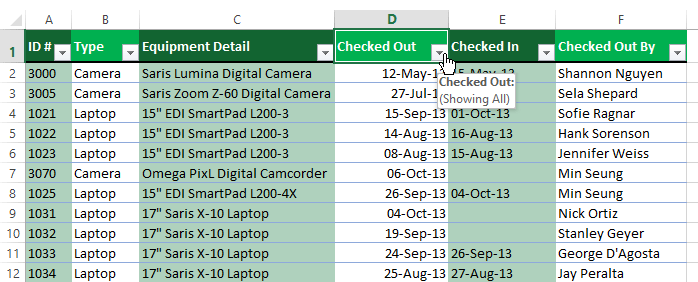
Click the drop-downwards arrow for the column you want to filter. In our instance, we will filter column D to view only a certain range of dates.
Clicking the drop-down pointer for cavalcade D
The Filter card will announced. Hover the mouse over Date Filters, so select the desired date filter from the drop-downwards menu. In our example, we'll select Today to view equipment that has been checked out on today's date.
Selecting a appointment filter
The worksheet will exist filtered by the selected appointment filter. In our example, nosotros can now see which items have been checked out today.
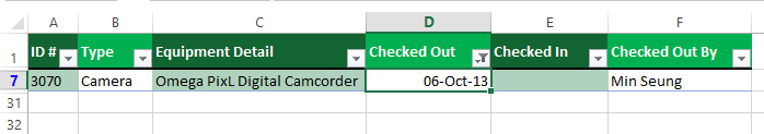The applied appointment filter

If yous're working along with the example file, your results will be different from the images to a higher place. If you want, y'all tin can change some of the dates so the filter will give more than results.

To employ advanced number filters:

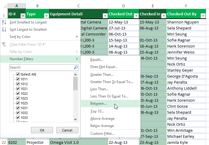
Advanced number filters allow you lot to dispense numbered data in different ways. In this example, nosotros will display only certain types of equipment based on the range of ID numbers.

Select the Data tab on the Ribbon, then click the Filter control. A drop-down arrow volition appear in the header cell for each cavalcade. Notation: If you've already added filters to your worksheet, y'all can skip this step.
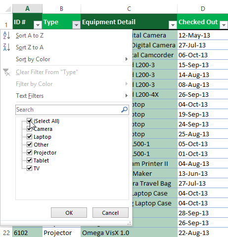
Click the drop-down arrow for the column you want to filter. In our example, we'll filter column A to view only a certain range of ID numbers.
Clicking the driblet-downward arrow for column A
The Filter bill of fare will announced. Hover the mouse over Number Filters, then select the desired number filter from the driblet-downward menu. In our example, we volition choose Between to view ID numbers between a specific number range.
Selecting a number filter
The Custom AutoFilter dialog box will appear. Enter the desired number(s) to the right of each filter, then click OK. In our example, we desire to filter for ID numbers greater than or equal to 3000 just less than or equal to 4000, which volition display ID numbers in the 3000-4000 range.

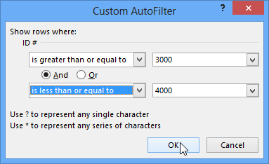Applying a number filter and clicking OK
The data will be filtered by the selected number filter. In our case, only items with an ID number between 3000 and 4000 are visible.

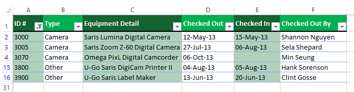The applied number filter

Challenge!

Open an existing Excel workbook. If you lot desire, you can utilize our practice workbook.
Apply a filter to a column. If you are using the example, filter the Type column (cavalcade B) and so it displays merely laptops and cameras.
Add another filter by searching. If y'all are using the instance, search for EDI brand equipment in the Equipment Item column (column C).
Clear both filters.
Use an advanced text filter to view data that does not contain a certain word or phrase. If y'all are using the example, display data that does not contain the word saris (this should exclude all Saris make equipment).
Use an advanced date filter to view data from a sure time menstruum. If y'all are using the example, display only the equipment that was checked out in September 2013.
Use an advanced number filter to view numbers less than a certain corporeality. If you are using the example, display all items with an ID# below 3000.

/en/excel2013/groups-and-subtotals/content/